Democratizing DeFi Research Part II: Deep Dive into Implied Volatility

Executive Summary
In this second installment of our three-part series on Democratizing DeFi Research, Doctor C gives us a deep dive into the open-source Python script used for studying implied volatility and volatility smiles of Uniswap Liquidity Providers (LPs).
We aim to unpack these complexities, enabling you to understand and use our code more effectively. This blog post doesn't just offer insights — it gives you the tools to conduct your own DeFi research and contribute to our growing body of knowledge.
Objectives
- Understand and pull from the Uniswap v3 subgraph
- Discover the relationship between LPs and implied volatility
- Create visual graphs of implied volatility smiles
Prerequisites
- Basic coding knowledge
- Basic familiarity with Python
As you gain a better understanding of how to use, replicate, and contribute to our open-source code, we hope you'll be empowered to run your own research and investigations.
Doctor C's Pick: Implied Volatility & Volatility Smile
Introducing the Script
This script is from our Research Bite on implied volatility and the volatility smiles. The script is particularly interesting because it extracts info from the Uniswap graph and demonstrates the relationship between implied volatility and LP sentiment.
In a nutshell, this code:
- Uses the Uniswap v3 subgraph to compute the amount of liquidity deployed to each tick in a given pool
- Converts the liquidity into a common currency (USDC, ETH, etc.)
- Computes the implied volatility based on the formula below
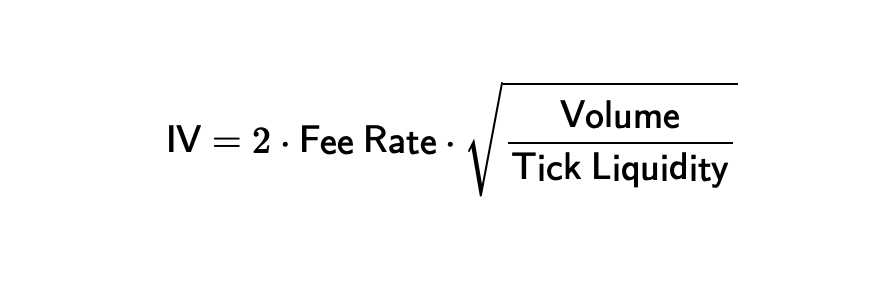
Implied volatility of a pool. Notice that this typically needs to be annualized (multiply by ).
Step By Step Breakdown
Before starting, we recommend downloading the gql library and importing all these required libraries:
from gql import gql, Client
from gql.transport.requests import RequestsHTTPTransport
import math
import sys
import pandas as pd
import numpy as np
import matplotlib.pyplot as plt
plt.style.use('panoptic-dark-16_9.mplstyle')
Step 1: Start by defining the pool you want to use. For example, use the ETH-UNI-30bps pool on the POOL_ID field, as defined below. You can find other pool addresses by clicking on the respective pool here.
POOL_ID="0x8ad599c3a0ff1de082011efddc58f1908eb6e6d8"
Step 2: Define a GraphQL query named pool_query. This query is designed to fetch data about specific liquidity pools from the Uniswap v3 subgraph. The query requires one argument, $pool_id, which should be the unique identifier (ID) of the pool you're interested in.
Later, we will set this input argument to POOL_ID.
pool_query = """query get_pools($pool_id: ID!) {
 pools(where: {id: $pool_id}) {
    tick
    sqrtPrice
    liquidity
    feeTier
    volumeToken0
    volumeToken1
    token0 {
      symbol
      decimals
    }
    token1 {
      symbol
      decimals
    }
  }
}"""
Here's a brief breakdown of what each part of the query is requesting:
pools(where: {id: $pool_id})is the main part of the query. It's asking the database to return data on the pool with the providedpool_id.tick,sqrtPrice,liquidity,feeTierare fields requesting specific data on the identified pool. These include data such as the pool's current tick, square root price, liquidity, fee tier, and the trading volume of both tokens in the pool.token0andtoken1are fields are requesting data on the two tokens traded in the pool. For each token, this query returns its symbol (e.g., ETH for ethereum), and the number of decimals the token has (i.e., 18 for WETH, 6 for USDC, etc.). This information is useful when computing the liquidity in a common currency.
Step 3: Define another GraphQL query named tick_query which is designed to fetch specific data from the "ticks" associated with a particular liquidity pool in Uniswap v3. The tick_query accepts two parameters:
$num_skip: an integer that represents how many ticks should be skipped before starting to return the results. This is useful for implementing pagination.$pool_id: the unique identifier of the pool from which you're interested in getting the ticks.
tick_query = """query get_ticks($num_skip: Int, $pool_id: ID!) { ticks(skip: $num_skip, where: {pool: $pool_id})
{ tickIdx liquidityNet } }"""
Here's what the query is requesting:
ticks(skip: $num_skip, where: {pool: $pool_id})asks for the ticks associated with the specified pool, skipping a certain number of them as defined by$num_skip.tickIdxandliquidityNet. For each tick, the query requests the tick index (tickIdx) and the net change in liquidity (liquidityNet) at that tick. The tick index refers to the specific price point that the tick represents, and the net liquidity represents how much liquidity was added or removed at that price point.
This is the script used to extract the liquidity on each tick in the pool.
Step 4: Define auxiliary functions to simplify some steps.
TICK_BASE = 1.0001
def tick_to_price(tick):
    return TICK_BASE ** tick
# Not all ticks can be initialized.
# Tick spacing is determined by the pool's fee tier.

def fee_tier_to_tick_spacing(fee_tier):
    return {
    100: 1,
    500: 10,
    3000: 60,
    10000: 200
    }.get(fee_tier, 60)
Step 5: Now use the following Python script to submit our queries to the Uniswap v3 subgraph. First, it attempts to execute the pool_query (which is a GraphQL query we discussed earlier) using the client's execute method, passing in the query and the variables. Then, it checks the response for the requested pool data.
If the response doesn't contain any pool (i.e., the length of response['pools'] is 0), it prints "pool not found" and exits with an error status. If the pool is found, it extracts the first pool from the response and assigns it to the variable pool. It then extracts the following pieces of data from the pool object:
tick(int) Current tick of the pool (i.e., price)Liquidity(int) Liquidity in the poolFeeTier(int) Fee tier of the pooltoken0(str) &token1(str) The symbol of each tokendecimals0(int) &decimals1(int) The number of decimals for each token
If any error occurs during this process (e.g., the query fails, the pool ID is invalid, or the data can't be extracted from the response), it catches the exception, prints an error message along with the exception details, and exits with an error status.
# Connects to the UniV3 subgraph
client = Client(
    transport=RequestsHTTPTransport(
    url='https://api.thegraph.com/subgraphs/name/uniswap/uniswap-v3',
    verify=True,
    retries=5,
))
# creates the pool dictionary
try:
    variables = {"pool_id": POOL_ID}
    response = client.execute(gql(pool_query), variable_values=variables)
    if len(response['pools']) == 0:
        print("pool not found")
        exit(-1)
    pool = response['pools'][0]
    current_tick = int(pool["tick"])
    tick_spacing = fee_tier_to_tick_spacing(int(pool["feeTier"]))
    token0 = pool["token0"]["symbol"]
    token1 = pool["token1"]["symbol"]
    decimals0 = int(pool["token0"]["decimals"])
    decimals1 = int(pool["token1"]["decimals"])
except Exception as ex:
    print("got exception while querying pool data:", ex)
    exit(-1)
Step 6: Once this data is computed, we query the liquidity on each tick in the Uniswap v3 pool of interest. It uses information such as the current tick, tick spacing, and the number of decimals each token uses obtained above.
This long script does several tasks:
Task 1: It initializes liquidity to 0, which is used to accumulate the total liquidity across all relevant ticks. It also initializes total_amount0 and total_amount1 to 0, which accumulates the total number of each token in the pool. Lastly, it calculates the minimum and maximum tick from tick_mapping, a dictionary that presumably maps each tick to the net change in liquidity at that tick.
def get_price_and_liq():
    # Step 6.1
    # Start from zero; if we were iterating from the current tick, would start from the pool's total liquidity
    liquidity = 0
    total_amount0 = 0
    total_amount1 = 0
    L=[]

    # Find the boundaries of the price range
    min_tick = min(tick_mapping.keys())
    max_tick = max(tick_mapping.keys())
Task 2: It calculates the bottom tick of the current range by flooring the division of the current tick and the tick spacing, then multiplies the result by the tick spacing.
# Step 6.2 It calculates the bottom tick of the current range by flooring the division of the current tick and the tick spacing, then multiplying the result by the tick spacing.p 6.2
# Compute the tick range. This code would work as well in Python: `current_tick // tick_spacing * tick_spacing`
# However, using floor() is more portable.
current_range_bottom_tick = math.floor(current_tick / tick_spacing) * tick_spacing
Task 3: It calculates the current price using the function tick_to_price() defined above, and adjusts it by dividing by 10 ** (decimals1 - decimals0).
# Step 6.3
current_price = tick_to_price(current_tick)
adjusted_current_price = current_price / (10 ** (decimals1 - decimals0))
Task 4: It decides whether to invert the price display based on the types of tokens and the adjusted current price. The goal is to display prices in terms of USD where possible.
# Sum up all tokens in the pool

# Step 6.4
# Guess the preferred way to display the price;
# try to print most assets in terms of USD;
# if that fails, try to use the price value that's above 1.0 when adjusted for decimals.
stablecoins = ["USDC", "DAI", "USDT", "TUSD", "LUSD", "BUSD", "GUSD", "UST"]
if token0 in stablecoins and token1 not in stablecoins:
    invert_price = True
elif adjusted_current_price < 1.0:
    invert_price = True
else:
    invert_price = False

# Iterate over the tick map starting from the bottom
tick = min_tick
ticks=[]
Task 5: It enters a loop to iterate over each tick from the minimum to the maximum tick. At each tick it calculates the liquidity, price, and amount of each token potentially in the range or actually in the range (if the tick equals the current range's bottom tick), and updates the total amounts of tokens accordingly.
# Step 6.5
while tick <= max_tick:
    liquidity_delta = tick_mapping.get(tick, 0)
    liquidity += liquidity_delta

    price = tick_to_price(tick)
    adjusted_price = price / (10 ** (decimals1 - decimals0))
    if invert_price:
        adjusted_price = 1 / adjusted_price
        tokens = "{} for {}".format(token0, token1)
    else:
        tokens = "{} for {}".format(token1, token0)

    should_print_tick = liquidity != 0
    #if should_print_tick:
       # print("ticks=[{}, {}], bottom tick price={:.6f} {}".format(tick, tick + tick_spacing, adjusted_price, tokens))

    # Compute square roots of prices corresponding to the bottom and top ticks
    bottom_tick = tick
    top_tick = bottom_tick + tick_spacing
    sa = tick_to_price(bottom_tick // 2)
    sb = tick_to_price(top_tick // 2)

    if tick < current_range_bottom_tick:
        # Compute the amounts of tokens potentially in the range
        amount1 = liquidity * (sb - sa)
        amount0 = amount1 / (sb * sa)

        # Only token1 locked
        total_amount1 += amount1
        # step 6.5.1
        if should_print_tick:
            adjusted_amount0 = amount0 / (10 ** decimals0)
            adjusted_amount1 = amount1 / (10 ** decimals1)
            cp=1 / adjusted_current_price if invert_price else adjusted_current_price
            print('current price')
            print(cp)
            #print("        {:.2f} {} locked, potentially worth {:.2f} {}".format(adjusted_amount1, token1, adjusted_amount0, token0))
            L.append(adjusted_amount1*cp)
    elif tick == current_range_bottom_tick:
        # Always print the current tick. It normally has both assets locked
        # Print the real amounts of the two assets needed to be swapped to move out of the current tick range
        current_sqrt_price = tick_to_price(current_tick / 2)
        amount0actual = liquidity * (sb - current_sqrt_price) / (current_sqrt_price * sb)
        amount1actual = liquidity * (current_sqrt_price - sa)
        adjusted_amount0actual = amount0actual / (10 ** decimals0)
        adjusted_amount1actual = amount1actual / (10 ** decimals1)
        L.append(adjusted_amount1actual*cp+adjusted_amount0actual)

        total_amount0 += amount0actual
        total_amount1 += amount1actual


    else:
        # Compute the amounts of tokens potentially in the range
        amount1 = liquidity * (sb - sa)
        amount0 = amount1 / (sb * sa)

        # Only token0 locked
        total_amount0 += amount0

        if should_print_tick:
            adjusted_amount0 = amount0 / (10 ** decimals0)
            adjusted_amount1 = amount1 / (10 ** decimals1)
            L.append(adjusted_amount0)
            #print("        {:.2f} {} locked, potentially worth {:.2f} {}".format(adjusted_amount0, token0, adjusted_amount1, token1))
    ticks.append(tick)
    tick += tick_spacing
Task 5.1: Inside the loop, the function decides to print the tick information based on whether the liquidity at that tick is non-zero. Then, it adjusts the amounts of tokens and appends them to a list L.
# step 6.5.1
if should_print_tick:
    adjusted_amount0 = amount0 / (10 ** decimals0)
    adjusted_amount1 = amount1 / (10 ** decimals1)
    cp=1 / adjusted_current_price if invert_price else adjusted_current_price
    print('current price')
    print(cp)
    #print("        {:.2f} {} locked, potentially worth {:.2f} {}".format(adjusted_amount1, token1, adjusted_amount0, token0))
    L.append(adjusted_amount1*cp)
Task 6: After the loop, the function calculates the price at each tick and returns it along with the array version of the list L.
# Step 6.6
price=1/(1.0001**np.array(ticks)*1e-12)

return price,np.array(L)
This function is then used to understand the distribution of liquidity across different price points in a liquidity pool and to calculate how much of each token is locked at each tick.
With these tasks defined, one step remains.
Step 7. Lastly, we compute the liquidity at different prices (i.e., call the previous function), and we plot the liquidity as well as the Implied Volatility (IV) from the formula above.
VOL=10.7e6 # volume in 24h, can get from query or from info.uniswap
BPS=10000
current_price=1/(1.0001**current_tick*10**(decimals0-decimals1))
lp=L[price[:-1]<1e4]
pp=price[price<1e4]
fee_tier=tick_spacing/(2*BPS)
IV=2*fee_tier*(VOL/lp)**0.5*(365)**0.5

# plots liquidity
fig, ax1 = plt.subplots()

ax1.stairs(lp/1e6,pp,label='Value locked (in USDC)')
ax1.set_xlim([500,5000])
plt.ylim([0,1.25])
ax1.set_xlabel('ETH price')
ax1.set_ylabel('USDC (millions)')
ax1.vlines(current_price,0,np.max(lp)/1e6,label='Current price, {} (USDC)'.format(round(current_price,2)),color='C1')
ax1.legend()
ax1.set_title('Value Locked & Volatility Smile, ETH-USDC-0.3%')

#plot IV on the right y-axis
ax2 = ax1.twinx()  # instantiate a second axes that shares the same x-axis
color='C2'
ax2.set_ylabel('Implied Volatility (%)', color=color)  # we already handled the x-label with ax1
ax2.plot(pp[:-1],IV*100, color=color) # multiply by 100 to get the %
ax2.tick_params(axis='y', labelcolor=color)
ax2.set_ylim([0,75])
fig.tight_layout()  # otherwise the right y-label is slightly clipped
plt.show()
Which should result in something like this:
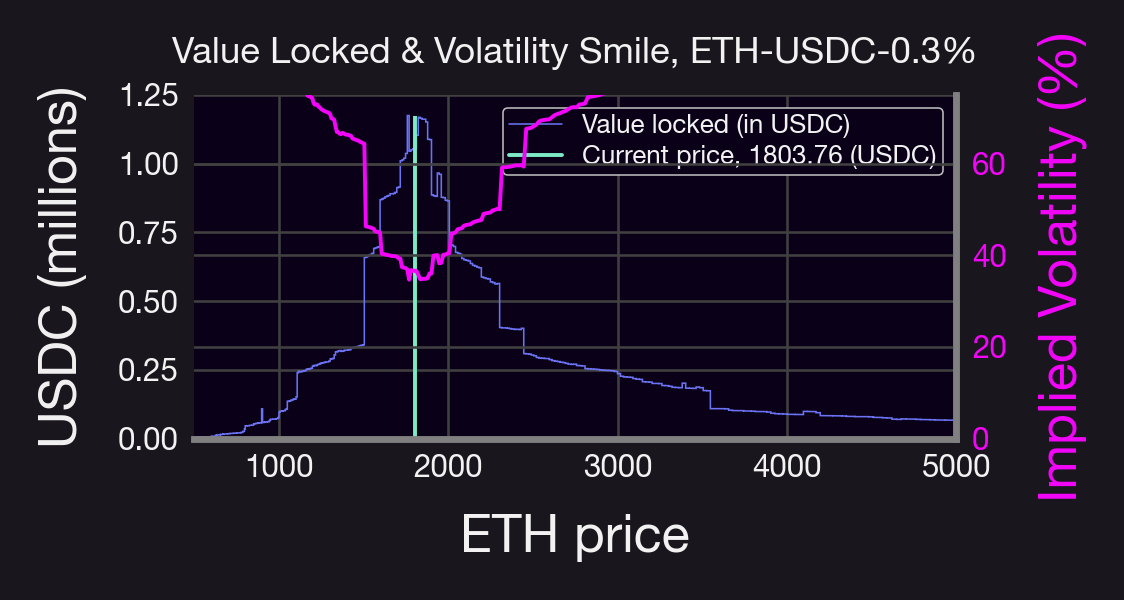
You can play around with the code once all the scripts are pieced together.
Upcoming Articles in the Series
In the final part of our series, we'll guide you through a comprehensive exploration of the Panoption backtester, another instrumental tool in our open-source arsenal.
Join the growing community of Panoptians and be the first to hear our latest updates by following us on our social media platforms. To learn more about Panoptic and all things DeFi options, check out our docs and head to our website.
Disclaimer: This is never financial advice, and you must do your own research at all times (DYOR). This content is provided free of charge and solely for educational reasons.